Synthetic Data for Aligning ML Models to Business Value

I improved a model to save a hypothetical auto insurance company almost $200 per claim!

One of the biggest mistakes that junior data scientists make is focusing too much on model performance while remaining naive about the model’s impact on the business. They implement costly model selection and hyper parameter optimization pipelines without thinking about whether the performance metrics that they’re using (e.g. accuracy, f1, etc) are actually aligned with what their employers need. As data scientists mature, they learn to spend less time training models and more time asking questions of the business, to ensure that they’re solving the right problems.

Synthetic data can be used by data scientists of all experience levels to not only improve model performance but also to help align the model to business value. With synthetic data, data issues (e.g. class imbalance, missing values, small datasets) can be remedied and models can solve important problems for businesses. To demonstrate this, I trained two RandomForest models with identical hyper-parameters: one on a raw dataset and the other on the same dataset augmented with synthetic data. When evaluated against the same test dataset, the augmented model performed almost 60x better on a custom business metric! This translated into $195.01 per data point!

To see how I was able to generate this synthetic data quickly and easily using YData Fabric, read on.

Data exploration

According to the FBI, fraudulent insurance claims cost American citizens approximately $40 billion annually. These fraudulent claims take many forms, from staged accidents to inflated claims and false reports of theft or damage. Detecting these fraudulent claims can be challenging, but advancements in technology and data analysis have led to the development of machine learning algorithms that can help identify patterns and anomalies that may indicate fraud.

I used the publicly available Vehicle Insurance Fraud Detection dataset from Kaggle to train my fraud detection models. Before cleaning this data or training any models on it, I used YData Fabric’s graphical user interface to explore my dataset. You can try out this feature of Fabric with a free trial account. Performing this type of exploratory data analysis (EDA) helps me understand the shape of my data and detect any potential issues with it.

Initial impressions

After uploading my dataset to the platform, I’m able to immediately see lots of insights about my data at a glance.

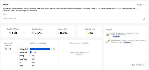
YData Fabric Data Catalog overview page

YData Fabric offers a rich UI with lots of useful information about my data, including automatically identifying potential issues with the data:

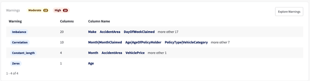
YData Fabric Catalog warnings section

Class imbalance

In fact, one particular issue is especially troubling:

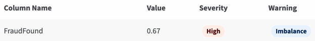
YData Fabric Catalog Imbalanced warning

We can see more details about this variable in the Profiling tab:

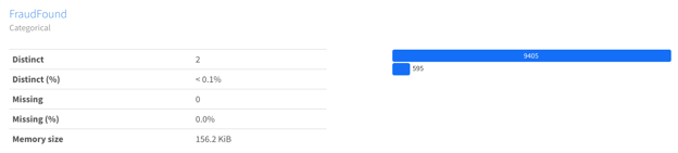
YData Fabric Catalog 'FraudFound' variable detail

With only 595 instances of fraud in a dataset of 15,000 rows, this is a very extreme example of class imbalance. This gives us a hint that synthetic data may be very powerful at improving the performance of models trained on this dataset, by balancing the classes.

Correlations

Another set of issues that indicates a problem with the dataset is the high number of correlation warnings. We can filter down the warnings to only show warnings about correlations:

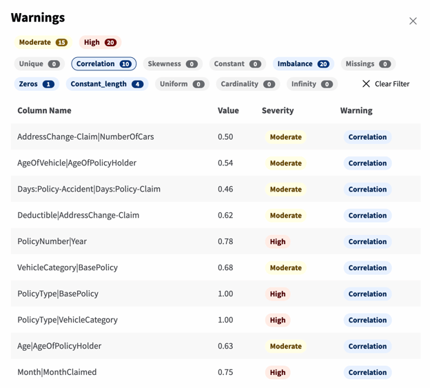
YData Fabric Catalog Imbalanced warning

Surfacing these types of correlations is useful because certain model types suffer from multi-collinearity, where model parameters swing wildly in response to slight perturbations in data. Although the RandomForest models we plan to train don’t suffer from multi-collinearity, their features become difficult to interpret when input variables are highly correlated.

In our situation, since our priority is only on performance and not on interpretability, we can safely use this dataset without removing highly-correlated features. However, it’s still useful to know that this feature exists, in case we want to train other models to be interpretable in the future.

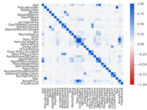
YData Fabric Catalog Correlation Matrix

Data Type

Finally, we can easily identify another potential issue with our data, specific to our RandomForest models. The sklearn implementation of the RandomForest algorithm can't have categorical data as inputs, so we’ll need to make sure that our dataset doesn’t have any categorical features. Otherwise, we’ll need to encode those variables during the data preparation stage.

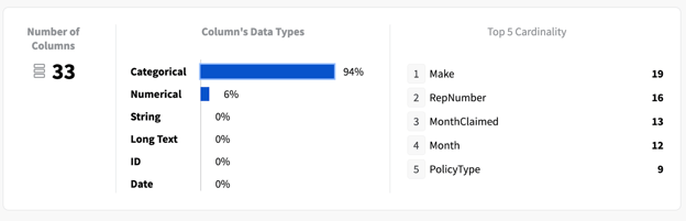
YData Fabric Catalog dataset variables overview

As it turns out, most of the input data columns are categorical! We’ll need to address this as part of our data preparation.

Data preparation

Now that we’ve identified the preparation that this data needs, we can go ahead with getting it ready first for synthesis and then for model training and evaluation. We’ll divide our data preparation into three steps:

• Defining functions for encoding categorical variables
• Importing the dataset and applying these functions
• Splitting the data into input and target variables, and then into training and testing sets

To keep following along, you’ll either need to request access to YData Fabric’s Labs feature or switch over to a Python IDE, such as a Jupyter Notebook, PyCharm, or VS Code.

Defining

We need to define two functions for encoding categorical variables: one for our target variable (FraudFound) and one for our input variables.

Defining a function for encoding the target variable is quite easy, since it only has two values. We want to encode “No” to be represented as 0 and “Yes” to be represented as 1. We can do this with the following code snippet:

Encoding our input variables is more complicated than the target variable. There are seemingly endless blog posts discussing which encoding techniques to use and when. Kaggle even had an immensely popular competition to compare different encoding methods. For the sake of simplicity, we are going to use target encoding because it doesn’t create an excess of new columns, is highly performant, and straightforward to implement. We’ll need to import the  'category_encoders' library, so make sure to have it installed.

Applying

After we’ve defined our data preparation functions, we can import our data and apply them:

Splitting

Now that we’ve got our 'car_claims_prepared' DataFrame, we can use sklearn’s train_test_split to split our data into training and testing, so that we can evaluate model performance. It’s important to do this step before data synthesis to prevent data leakage—where testing data is included in the synthesis of new data—and prevent synthetic data from making its way into the testing set.

Before we can split our data, however, we need to separate the input variables from the target variable. This is important because, when fitting our RandomForest estimator, we need to pass the input and target variables as separate arrays.

Fortunately, this is all easy to do with a few lines of code:

Data synthesis

Now that we’ve got our dataset prepared, we can move on to synthesizing new data to add to the training set to create an augmented dataset. Recall that we are specifically looking to fix the class imbalance in our target variable, so we’ll rely on YData’s Conditional Sampling feature to only generate observations where fraud was detected. 

Presently, conditional sampling is only available for users in Labs, so if you’ve been following along in a Python IDE you’ll need to generate a larger amount of synthetic data using the Fabric SDK or GUI, and then filter out synthesized data where FraudFound == 0. The easiest way to follow along is to contact us for access to the Labs feature.

Before creating a Synthesizer, we’ll need to create a single training dataset that contains both our input variables as well as our target variable and save it as a CSV. As discussed above, we’ll want to avoid having our test data in the data used by the Synthesizer, to prevent data leakage. Fortunately, this is easy to do with Pandas:

Now that we’ve got our training dataset saved locally, we can create a Fabric Dataset from it. Let’s start by importing the modules that we’ll need and then create a Fabric Dataset from the CSV file we just created:

Next, we can easily create a Synthesizer and fit it to the dataset. This trains a generative model based on our dataset. We need to specify that we will be creating data conditioned on the target feature class, which we can specify with the `condition_on` parameter:

Now that we’ve created our Synthesizer, we can generate synthetic data to augment our dataset and balance our classes. We can determine the number of data points that we want to generate by subtracting the number of data points with fraud from the number of data points without fraud in the training dataset. Once we’ve calculated that difference, we can generate our new data:

Finally, we can append this data to a copy of our training dataset, creating an augmented training dataset:

Model training

With all of the setup that we’ve done, training our models will be very straightforward. We will use sklearn’s RandomForestClassifier algorithm with default hyperparameters to train a first model based on the raw data and a second model based on the augmented data. After training each model, we’ll make predictions for each of the data points in the testing set.

First, let’s train our model based on the raw dataset:

And now on the augmented dataset:

Model evaluation

Now that we’ve got our fitted models and their predictions, we can evaluate them. We’ll do this by defining a series of functions and then executing those functions with each model’s predictions.

Definitions

We’ll define functions to output:

• Performance metrics for each model
• A confusion matrix for each model’s predictions
• A prediction of business value for each model
  

Performance metrics

First, let’s define a function to derive key performance metrics about the models. In this case, I’ve decided to examine the f1 and recall of the models, but you could conceivably choose to concentrate on other performance metrics. I used sklearn’s built-in performance metrics module to do this:

Confusion matrix

In addition to the performance metrics, I find it helpful to visualize the predictions and actuals of my test set using a confusion matrix. Confusion matrices are helpful for quickly understanding where model prediction errors are happening and what class or classes a model might be underperforming in. I copy/pasted some standard code to use matplotlib and Seaborn for generating a confusion matrix based on predictions and actuals:

Business value

Finally, and most interestingly, I wanted a business value evaluation for each model. I defined two functions: a main business_value function and a business_score helper function.

The business_score function takes in actuals and predictions and outputs an estimated “cost per claim” of the model. The first step to generate this “cost per claim” is calculating the count of false positives (where the model predicts fraud even though no fraud has occurred) and false negatives (where the model predicts no fraud even though there actually was afraid). Once these two counts are calculated, they can be multiplied by two constants: the false positives by the estimated cost of a false positive and the false negatives by the estimated cost of a false negative. I estimated the cost of a false positive (where a claim is incorrectly rejected) to be $500, based on an estimate that an incorrectly identified case of fraud would take around 10 hours for a fraud investigator to solve and that they’d be paid $50/hour. I estimated the cost of a false negative (where fraud is allowed to slip by) as $5,700, which is the average cost of vehicle repair after an accident, according to the National Safety Council. These are very rough estimates and I’m sure that someone with experience in the auto insurance industry could help refine these numbers, but they seem like a good place to start for estimating the impact of synthetic data.

Multiplying the counts of each error by the corresponding costs results in the total cost for each type of error. Adding the products together results in a total cost, which is an estimate of how much the model’s errors are costing the business compared to a perfect model. Dividing this total cost by the number of claims gives us an average cost per claim, which I treat as a business score.

After generating this business score, we can further generate a business value for each model by comparing the cost of a model with the cost of a “naive” model. In this case, the naive model predicts every claim to not be fraudulent, since that will result in it being correct most of the time. By subtracting the business score of a model from the business score of this naive model, we can see how much money the model is saving the business compared to using a naive model. This tells us how much value the data scientist has created for the business:

Evaluations

Now that our models are trained and our functions for evaluating the models are defined, we can begin to evaluate the two models and see how they perform in terms of performance metrics, their confusion matrices, and the business value that each provides. We’ll evaluate first the model trained on the raw dataset and then the model trained on the augmented one.

Raw dataset

With the predictions made by the first model and the ground truths of the test set, we can evaluate our first model:

This outputs:

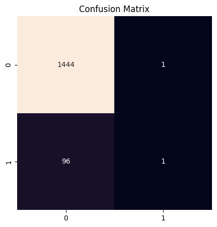
Classifier confusion matrix for the raw dataset

As we can see, the f1 score and recall for this model were quite low, around 0.02 and 0.01 respectively. Although the model would save an average of $3.37 per claim compared to a naive model, it only correctly identified a single instance of fraud. It was very good at correctly identifying non-fraudulent claims as non-fraudulent, but it missed 96 instances of fraud, costing the company $547,200 just from fraud in the testing set.

Augmented dataset

Similarly, we can use the predictions made by the model trained on the augmented dataset to evaluate our second model:

Which outputs:

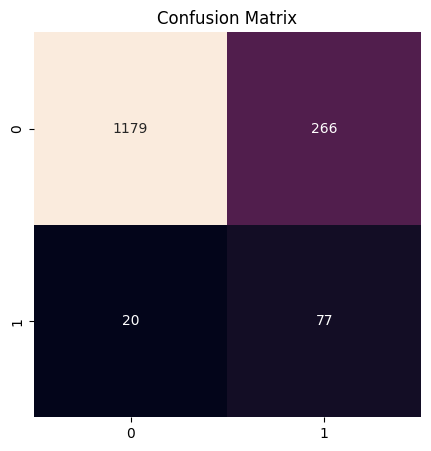
Classifier confusion matrix for the augmented dataset

Here, we see a significant improvement in both the f1 score and the recall of the model. The f1 score improved from ~0.02 to 0.35, a more than 17.5x improvement. And the precision improvement was even more dramatic, from ~0.01 to ~0.79, a 79x improvement. Because the model correctly predicted 77 out of 97 instances of fraud in the dataset, it would save the company an average of $198.38 per claim.

Model comparison

Finally, after having evaluated both models, we can compare their performances.

It’s easy to see that the f1 score of the augmented model is a significant improvement compared to the model trained on raw data, but this metric won’t be meaningful to business stakeholders. To justify the value of synthetic data, we need to show how synthetic data improves the model’s ability to save the company money on fraudulent claims. We can do this by comparing the business value of the two models against each other, finding both the difference and the quotient:

This outputs:

As we can see, using the model trained on synthetic data is a significant improvement compared to the model trained on raw data. Importantly, this lift came with very little effort on the part of the data scientist, so they have lots of time to continue to refine the model by doing more extensive data collection and feature engineering, evaluating different model architectures—logistic regression and gradient boosted trees come to mind, but deep learning might perform well here too—and optimizing the hyperparameters of those models.

Overall, I was shocked by how powerful synthetic data was at improving performance for this use case. To see how easy it is to improve your own models with synthetic data, sign up for a free, limited-feature trial or contact us for trial access to the full platform.