A practical guide to generating synthetic data using open-sourced GAN implementations
The advancements in technology have paved the way for generating millions of gigabytes of real-world data in a single minute, which would be great for any organization or individual in utilizing the data. However, a large amount of time and resources would be consumed in cleaning, processing, and extracting vital information from the mounds of data.
The answer to handling such a problem is by generating synthetic data.
What is Synthetic Data?
The definition for synthetic data is quite straightforward: artificially generated data that mimics real-world data. Organizations and individuals can leverage the use of synthetic data to their needs and would be able to generate data, according to their specifications, as much as they require.
The use of synthetic data is highly beneficial in preserving privacy in information-sensitive domains: the medical data of the patients and transactional details of banking customers are a few examples where synthetic data can be used to mask the real data, which would enable sharing of sensitive data among organizations.
Few well-labelled data can be used to generate a large amount of synthetic data, which would fast-track the time and energy needed to process the massive real-world data.
There are many ways of generating synthetic data: SMOTE, ADASYN, Variational AutoEncoders, and Generative Adversarial Networks are a few techniques for synthetic data generation.
This article will focus on using Generative Adversarial Networks to generate synthetic data and a practical demonstration of generating synthetic data using open-sourced libraries.
A Brief Introduction to GANs
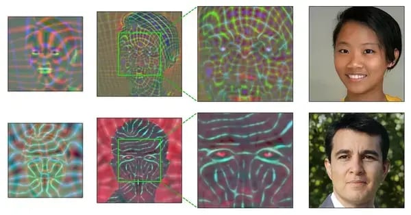
Generating photorealistic faces using GANs based on StyleGAN3 research. Image from [1].
Many machine learning and deep learning architectures are prone to adversarial manipulation, that is, the models fail when data that is different to the one that is used to train is fed. To solve the adversarial problem, Generative Adversarial Networks (GANs) were introduced by Ian Goodfellow [2], and currently, GANs are very popular in generating synthetic data.
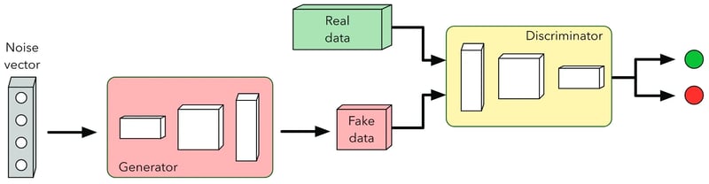
A typical GAN consists of two components: generator and discriminator, where both networks compete with each other.
The generator is the heart of the GAN, where it attempts to generate fake data that looks real by learning the features from the real data.
The discriminator evaluates the generated data with the real data and classifies whether the generated data looks real or not, and provides feedback to the generator to improve its data generation.
The goal of the generator is to generate data that can trick the discriminator.
A Vanilla GAN architecture. Image from [3].
Mode Collapse
Mode collapse is a common problem that GAN-based architectures face during adversarial training, where the generator repeatedly generates one specific type of data. This occurs when the generator identifies that it can fool the discriminator with one type of data, the generator would keep on generating that same data.
This problem can easily go undetected, as the metrics would indicate the model training is running smoothly, but the generated results would indicate otherwise.
An example of mode collapse in image-based GANs. Image from [4].
Wasserstein GAN (WGAN)
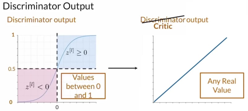
The main problem in a standard GAN is the difference in complexity of the outputs from the generator and the discriminator.
A standard Vanilla GAN uses the Binary Cross Entropy (BCE)loss function [5] to evaluate whether the generated data looks real, where the output of the loss function is between 0 and 1. The task of the generator is to generate synthetic data that might have a lot of features and values, and the output from the discriminator is not sufficient for the generator to learn, and due to the lack of guidance, the generator can easily fall into mode collapse.
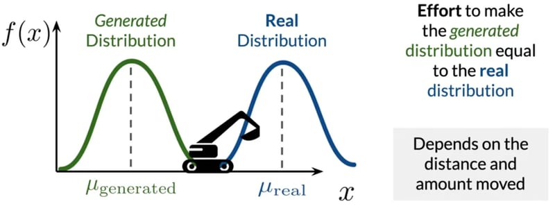
WGAN [6] alleviates the problem by replacing the discriminator with a critic, where the critic would evaluate the distribution of the real data with the distribution of the generated data and outputs a score of how real the generated data looks when compared to the real data. The Wasserstein loss function utilized in WGAN measures the difference between the real distribution and the generated distribution based on the Earth Mover’s Distance.
Visualization of Earth Mover’s Distance. Image from Coursera course [8]
Earth Mover’s Distance measures the effort that is needed to make the distribution of the generated data look similar to the real data’s distribution. Therefore, there is no limitation on the value that is output. That is, if both distributions are far apart, the Earth Mover’s Distance will give a real positive value, whereas the BCE loss would output gradient values that are closer to zero. Therefore, the Wasserstein loss function enables solving the vanishing gradient problem during training.
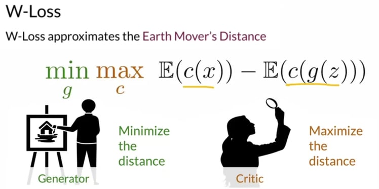
The expression of Wasserstein Loss. Image from Coursera course [8].
The above picture denotes the equation for the Wasserstein loss, which is relatively simple compared to the BCE loss. The initial part of the equation is the expected value of the prediction that the critic provides on the real data. The second part of the equation is the expected value of the prediction that the critic provides on the generated data. The goal of the critic is to maximize the distance between the real and generated data, and the goal of the generator is to minimize that difference.
Difference between BCE (left) and Wasserstein (right) losses. Image from Coursera course [8].
WGANs are prone to exploding gradient problems, as the Wasserstein loss outputs any value that is positive and real; therefore, the value of the gradients can uncontrollably increase when the distribution of the generated data differs from the real data’s distribution. This is solved by introducing a regularisation term, gradient penalty [7], which makes sure the gradients are contained, and this ensures better optimization of the WGAN model.
The ydata-synthetic library helps immensely in building GANs to generate synthetic data for tabular datasets, which otherwise would have been challenging and tedious.
There are a plethora of different types of GANs that can be used to generate synthetic data: the standard Vanilla GAN and Conditional GAN, and the advanced WGAN, WGAN with gradient penalty, Deep Regret Analytic GAN, CramerGAN, and Conditional WGAN, and a GAN option available for time series as well (TimeGAN).
The models can be used out-of-the-box with little modifications and can be used on almost any tabular dataset.
The library can be installed in the python environment with just one simple command:
pip install ydata-synthetic
The GitHub repository of ydata-synthetic
The Dataset
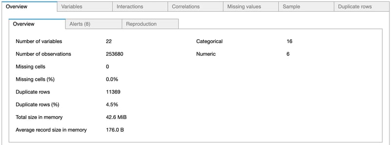
The Diabetes Health Indicators dataset is chosen, which is CC0 licensed. The dataset has sensitive data, which are medical records of patients, and there is a need to obtain more data regarding the patients diagnosed with diabetes; therefore, the use of synthetic data would be highly beneficial. The dataset consists of 21 features, and the target feature is whether the patient is diagnosed with diabetes.
Another open-sourced tool, ydata-profiling, is useful for exploratory data analysis, visualizing features and relationships with just two lines of code, and that tool is used to conduct the exploratory data analysis on the Diabetes Health Indicators dataset. This generates a detailed report on all the variables present in the dataset, alerts for any abnormalities present in the data, displays the relationship (or correlation) between variables, and shows the missing values in each column and the duplicates present in the data.
The GitHub repository for pandas-profiling
Loading the data and running pandas-profiling.
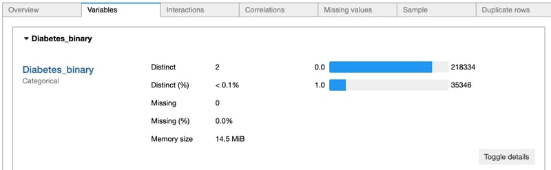
There are more than 218,000 examples of non-diabetes patients and more than 35,000 patients diagnosed with diabetes.
The number of patients with and without diabetes.
All the variables are of float type, as the dataset has undergone pre-processing. With the help of the pandas-profiling library, it was discovered that there are 3 numerical variables (BMI, MentHlth, and PhysHlth), and the other variables are categorical. The pandas-profiling tool highlighted that about 4% of the dataset comprises duplicates.
A general overview of the data.
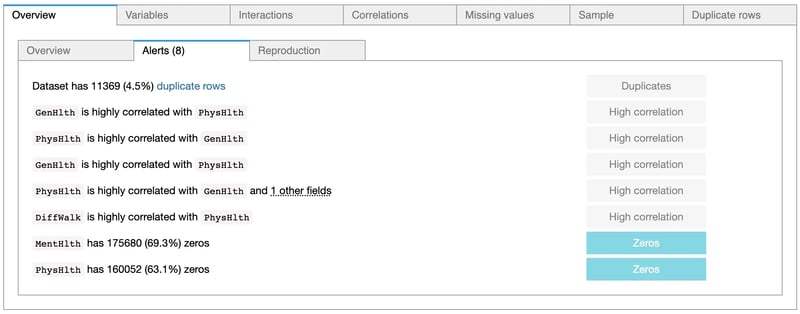
The pandas-profiling tool also highlighted highly correlated relationships between certain variables, which can be considered later for feature engineering tasks.
Abnormalities detected by the pandas-profiling library. Image from the author.
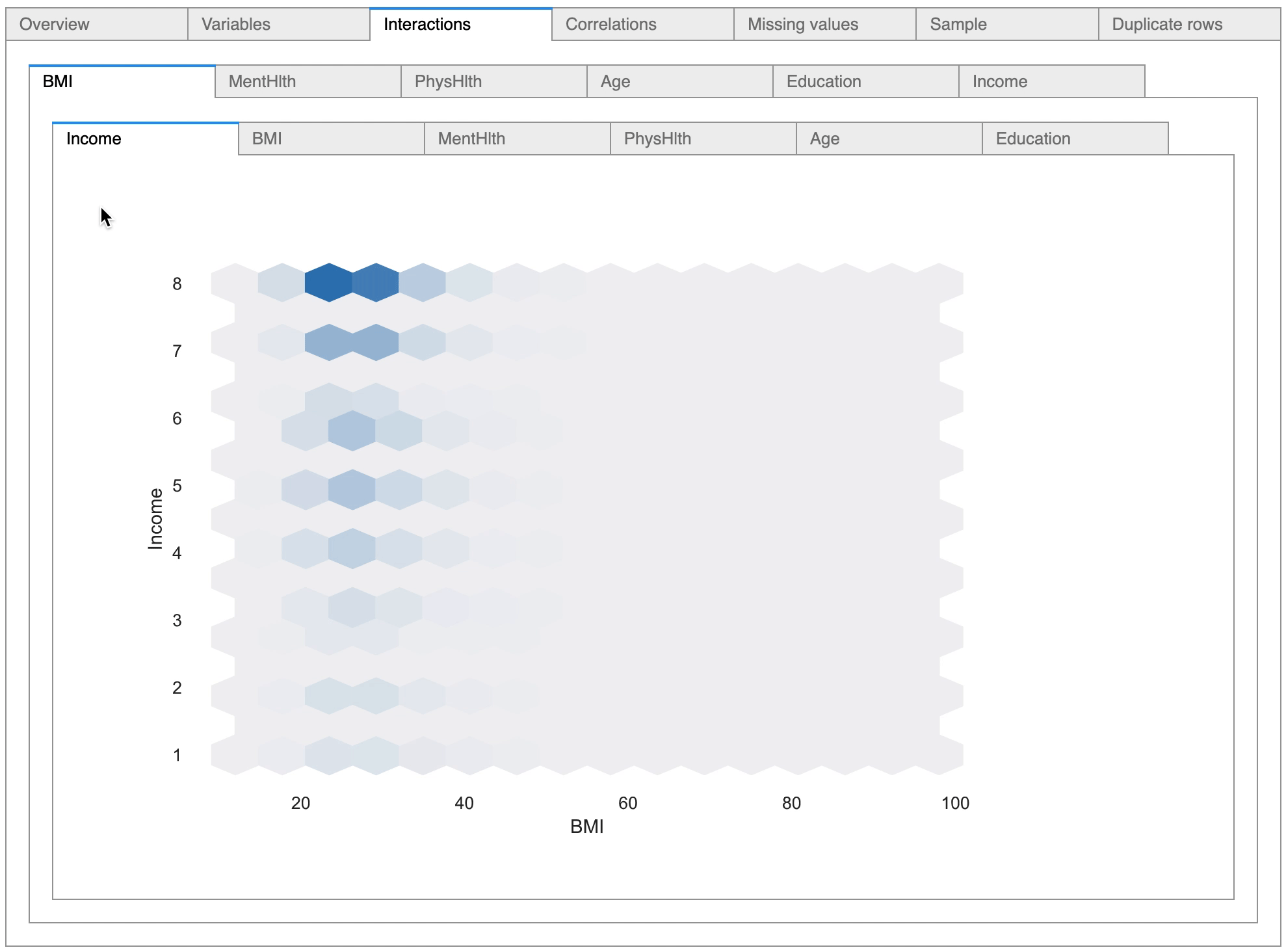
There are options to view the relationship between variables, and as can be seen in the above diagram, the pandas-profiling tool has detected six numerical variables and has plotted scatter plots depicting the relationship between the variables.
Viewing interactions between the numerical variables.
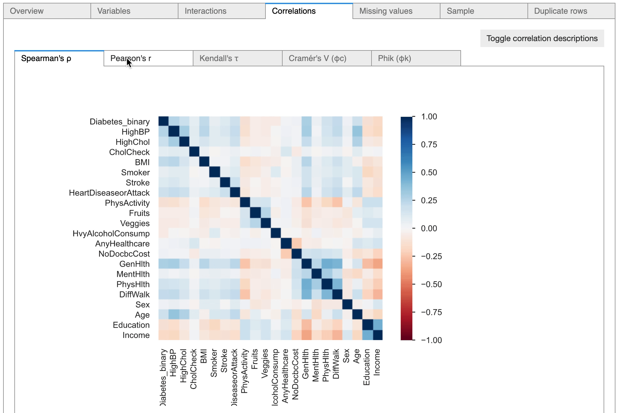
The tool is also highly useful in conducting statistical correlation tests between variables, as it provides options to conduct numerical correlation tests as well as categorical correlation tests.
Different correlation tests are available in the pandas-profiling library.
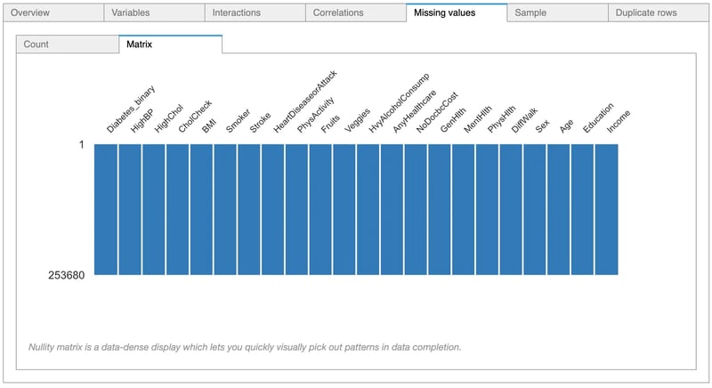
The pandas-profiling tool indicates that there are no missing values in the dataset.
No missing values are present in the data.
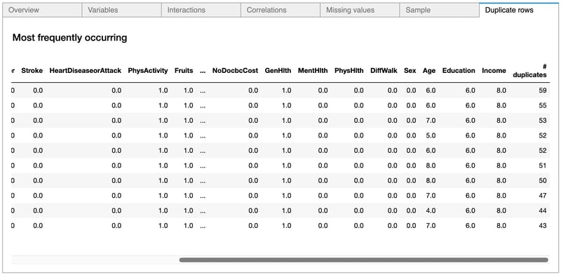
Since 4.5% of the data consists of duplicates, it is possible to check the exact duplicate rows and how many times such rows are repeated.
The duplicates that are present in the data.
Designing and Training the Synthesizer
Initially, the numerical and categorical columns are separated, as the type of variables is necessary to train the GAN model. Based on the data analysis that was done earlier, there are three numerical variables, and the rest are categorical variables.
To begin the process of generating synthetic data, the labels of the patients are separated based on their diabetic status. At first, a GAN is trained to generate synthetic data for patients who are diabetic.
Selecting the categorical and numerical variables, and selecting data with only diabetic patients.
The next step is to select the GAN model, and as discussed earlier, the Wasserstein GAN with Gradient Penalty is chosen. It is quite easy to initialize the GAN using the ydata-synthetic library.
Initializing the GAN model.
Once the GAN is initialized, the training process is initiated.
Starting the training process of the GAN.
The training time depends on the machine that is used for training. With an NVIDIA GPU, the training is much faster compared to training on the CPU. However, the library is also optimized to train well on the CPU.
Once the training is completed, the next step is to generate synthetic data. The GAN model is trained to understand the distribution of the data of diabetic patients, and 100,000 rows of data representing the diabetic patients are generated.
Generating synthetic data for diabetic patients.
Compared to the 35,000 rows of diabetic patients that are present in the original dataset, using a GAN-based model, 100,000 rows of synthetic data of the diabetic patients are available. And another advantage of using ydata-synthetic is that the synthetic data is returned in the form of the input data, with all the columns intact.
The steps for training the GAN on the majority class are similar to the previous steps taken to generate data for the minority class. The number of epochs to train the GAN for the non-diabetic patients’ data is set to 100 to reduce the training time.
Generating synthetic examples for non-diabetic patients’ data.
A simple code function is used to merge the synthetic samples of the majority and the minority classes.
Concatenating the synthesized majority and minority dataframes.
The pandas-profiling tool is used to obtain a quick exploratory data analysis of the synthetic data.
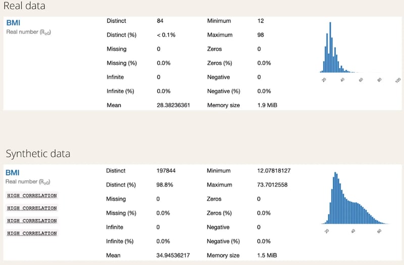
The distributions of the numerical columns from the real dataset and the generated dataset are evaluated.
Considering the BMI feature, the synthetic data has an acceptable representation of the real dataset. The range of values of the synthetic data is within the range of values of the real data. The mean of the synthetic data has shifted to the right, but overall, the BMI column of the synthetic data is comparable with the real data.
Comparison of BMI column with real and synthetic data.
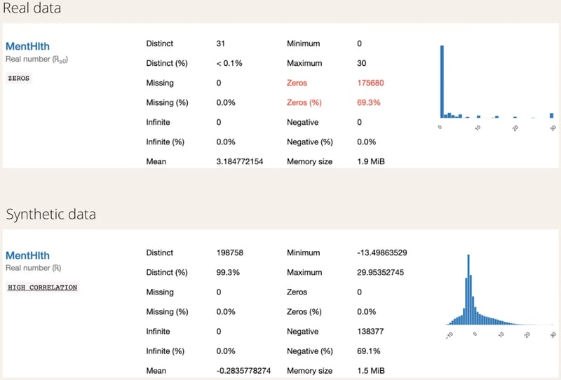
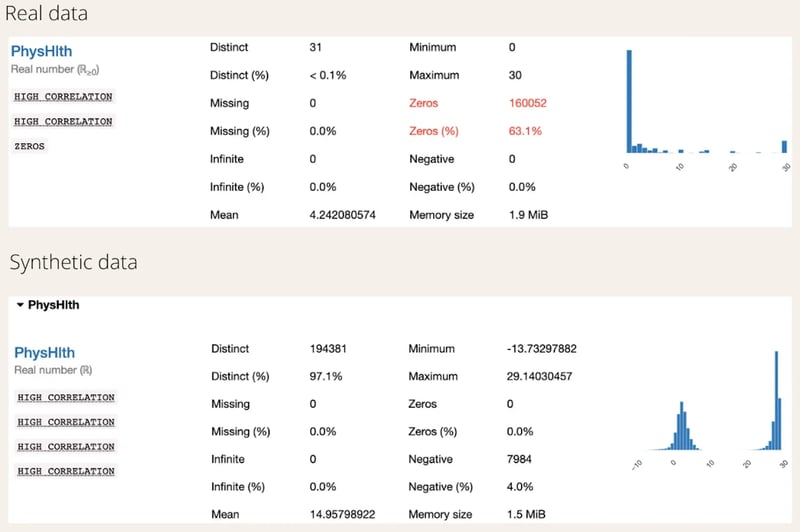
Comparing the “MentHlth” and “PhysHlth” can be a bit tricky. According to the definition of the columns based on the data, these two columns represent the number of days of poor mental health in the past 30 days and the number of days of a physical injury in the past 30 days, respectively. Therefore, a lot of values in these columns are zero, and the data is numerical, as the number of days is considered.
The synthetic data has generated negative values for the two columns, and this requires some feature processing before moving on to modelling, as the negative values would be converted to zeros.
When considering the feature “MentHlth”, the synthetic data has generated an acceptable distribution, as all the generated values are under 30. The mean of the synthetic data has shifted to the left.
Comparison of MentHlth column with real and synthetic data.
However, the mean of the synthetic data for the column “PhysHlth” has shifted significantly to the right. But the generated values are less than 30, and replacing the negative values with zero might slightly improve the generated results.
Comparison of PhysHlth column with real and synthetic data.
It is crucial to note that for the “PhysHlth” and “MentHlth” fields in the real data, nearly 70% of the values are zero. And for the remaining 30% are dispersed between 1–30, but not in any specific pattern. There is no specific distribution that can be seen in those two columns, unlike the “BMI” field. This would have been another important reason for the GAN to generate negative values for the “PhysHlth” and “MentHlth” fields.
There is a peak around the zero value in the distributions of the synthetic “PhysHlth” and “MentHlth” columns, which indicates the synthesizer has identified that a lot of values of both the columns are zero, but since both of those fields are initialized as numerical, the GAN is attempting to predict exact numeric values, and hence, negative values are generated.
The paradigm of AI is being transformed from model-centric to data-centric approaches, and the usage of synthetic data accelerates that transformation.
Synthetic data provides a low-cost and privacy-secured alternative to collecting and labelling real-world data, and anyone can utilize open-sourced powerful tools to generate data for their specific use cases.
There are many open-sourced tools available for generating quality synthetic data, and as discussed in this article, it is relatively easy to generate synthetic data by leveraging the power of GANs with the help of ydata-synthetic.
I hope you have learned how simple it is to generate synthetic data for tabular datasets, and looking forward to seeing how you will use these powerful tools to play with and create synthetic data. Cheers!
References
[1] T. Karras, S. Laine, and T. Aila, “A Style-Based Generator Architecture for Generative Adversarial Networks,” IEEE Transactions on Pattern Analysis and Machine Intelligence, pp. 1–1, 2020, doi: 10.1109/tpami.2020.2970919.
[3] G. H. de Rosa and J. P. Papa, “A survey on text generation using generative adversarial networks,” Pattern Recognition, vol. 119, p. 108098, Nov. 2021, doi: 10.1016/j.patcog.2021.108098.
[5] U. R. Dr A, “Binary cross entropy with deep learning technique for Image classification,” International Journal of Advanced Trends in Computer Science and Engineering, vol. 9, no. 4, pp. 5393–5397, Aug. 2020, doi: 10.30534/ijatcse/2020/175942020.
[7] I. Gulrajani, F. Ahmed, M. Arjovsky, V. Dumoulin, and A. Courville, “Improved Training of Wasserstein GANs,” arXiv:1704.00028 [cs, stat], Dec. 2017, [Online]. Available: https://arxiv.org/abs/1704.00028